The Shortest and Closest Vector Problems
The fundamental problems of lattice-based cryptography.
So far, we have only talked about properties and ways to describe lattices, but that doesn't inherently have anything to do with cryptography. This connection is made through hiding information by utilizing the structure of lattices. In other words, lattice-based cryptography relies on lattice problems, such as the shortest vector problem (SVP). SVP essentially asks questions surrounding finding the shortest vectors of a lattice given a basis.
Recall that there are an infinite number of bases that generate the same lattice. In previous blogs, we have given relatively "simple" bases, but that is not always the case. For instance, consider the basis \[ B := \begin{pmatrix} 3\sqrt{3898} & -5382\sqrt{\frac{2}{1949}} & \frac{31195}{\sqrt{3898}} & \frac{15857}{3}\sqrt{\frac{2}{1949}} \\ 0 & \sqrt{\frac{682378}{1949}} & -110727\sqrt{\frac{2}{664977361}} & \frac{676011}{\sqrt{1329954722}} \\ 0 & 0 & \sqrt{\frac{64221}{682378}} & \frac{67240}{3}\sqrt{\frac{2}{21911498769}} \\ 0 & 0 & 0 & \frac{1}{3\sqrt{128442}} \end{pmatrix}, \] which is borrowed from [1]. How would we interpret this? What is the shortest vector in the lattice formed by this basis? Since this is not immediately obvious (to a human, but computationally this is extremely weak and not secure), this is a bit more difficult than the bases we were previously using.
Minimum Distance
We need to collect some more lattice ``tools'' to analyze and understand SVP, especially what it means to have a shortest vector. We discuss some linear algebra machinery such as the Euclidean norm, sometimes denoted as the $\ell_2$ norm. More specifically, for some vector $x = (x_1, \ldots, x_n) \in \RR^n$, the $\ell_2$ norm is \[ \norm{x}_2 = (x_1^2 + \ldots + x_n^2)^{1/2}, \] essentially the ordinary geometric length from the origin to $x$. Sometimes other norms will be used too: \[ \norm{x}_p = (\lvert x_1\rvert^p + \ldots + \lvert x_n \rvert^p)^{1/p} \] for $p \geq 1$, but this is not as common. Assume we are using the Euclidean norm unless stated otherwise.
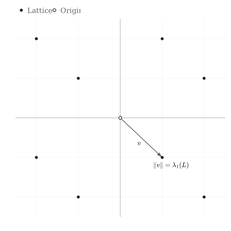
The minimum distance of a lattice $L$ is defined as \[ \lambda_1(L) := \min_{v \in L \setminus \{0\}} \lVert v \rVert = \min_{x,y \in L} \lVert x-y \rVert \] where $x \neq y$. In non-notation terms, it is the minimum non-zero norm of a vector within a lattice, which can be generalized to distinct vectors. Figure 1 shows how this works on a two-dimensional graph.
SVP
Let's define an approximate version of SVP, which can also be used for an exact version. The $\gamma$-approximate SVP, where $\gamma \geq 1$, is defined in three variants. This language is largely borrowed from [2], where we (somewhat) grossly simplify.
Decision
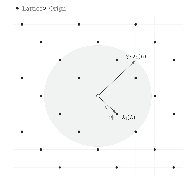
Decision ($\mathsf{GapSVP}_\gamma$) asks, given a lattice basis $B$ and a real $d > 0$, to distinguish between \[ \lambda_1 (L(B)) \leq d \text{ and } \lambda_1 (L(B)) > \gamma \cdot d \] The exact version $\mathsf{GapSVP}$ is when $\gamma = 1$. This asks us to tell whether $d$ is greater than or equal to the minimum distance, or (approximately) less than the minimum distance. Figure 2 shows how the problem looks by displaying this approximate problem as a ``ball.''
Estimation
Estimation ($\mathsf{EstSVP}_\gamma$) asks, given a lattice basis $B$, to compute $\lambda_1 (L(B))$ up to a $\gamma$ factor, meaning in the range \[ [\lambda_1 (L(B)),\ \gamma \cdot \lambda_1 (L(B))]. \] The exact version $\mathsf{EstSVP}$ asks us to calculate $\lambda_1 (L(B))$. This is asking us to calculate the (range of the) minimum distance.
Search
Search ($\mathsf{SVP}_\gamma$) asks, given a lattice basis $B$, to find a nonzero $v \in L(B)$ such that \[ \norm{v} \leq \gamma \cdot \lambda_1 (L(B)). \] The exact version $\mathsf{SVP}$ asks us to calculate $v$ such that $\norm{v} = \lambda_1(L(B))$. Essentially, it asks us to calculate the vector with the (approximate) minimum distance.
Discussion on hardness
While we will talk a bit more formally about hardness in a future post, it might be helpful to contextualize the differences between the problems. For now, it suffices to say that if you can solve the search problem, you can solve the other two problems. An intuitive way to think of this is that if you can calculate the shortest vector, you can compute $\lambda_1(L(B))$ (or the approximate version). Thus, you can solve the decision problem.
There are a few algorithms, historic and contemporary, that are common when speaking about calculating SVP. One example is the LLL algorithm [3], which approximates a short nonzero lattice vector. Additionally, a randomized sieving technique [4] solves SVP in $2^{O(n)}$ time and space. The contemporary discrete-Gaussian-sampling algorithm [5] solves it in $2^{n+o(n)}$ time and space. Note that the solving algorithms (not inherently LLL) are all exponential in $n$, meaning that there is no known polynomial or efficient algorithm.
CVP
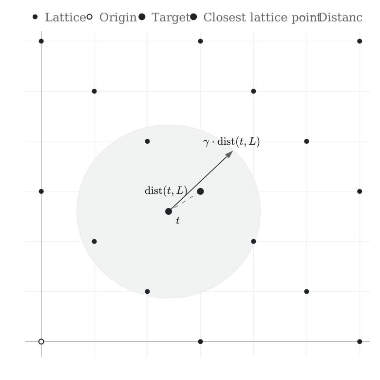
The Closest Vector Problem (CVP) is closely related to SVP. Rather than finding a shortest nonzero vector in a lattice, we are given some target $t \in \mathbb{R}^n$ and consider the distance between $t$ and the closest lattice point. We define this distance as \[ \dist{t,L(B)} = \min_{v \in L(B)} \norm{t-v}. \]
The decision, estimation, and search variants of CVP are defined similarly to their respective SVP variants, replacing $\lambda_1(L(B))$ with $\dist{t,L(B)}$. Thus, $\mathsf{GapCVP}_\gamma$ asks whether the target is within some distance $d$ of the lattice or farther than $\gamma d$. $\mathsf{EstCVP}_\gamma$ approximates $\dist{t,L(B)}$. $\mathsf{CVP}_\gamma$ finds a lattice vector whose distance from $t$ is within a factor $\gamma$ of the minimum possible distance, i.e., $\norm{t-v} \leq \gamma \dist{t,L(B)}$.
Intuitively, SVP asks us to find the shortest vector relative to the origin, while CVP lets us choose an arbitrary target and asks for the closest lattice point to that target. Although they are related, they are not the same problem. Figure 3 displays CVP graphically.
Discussion on hardness
As with SVP, the search version gives us enough information to solve the calculation and decision versions. Additionally, SVP can be solved using a CVP ``solver'' [6], so CVP is at least as hard as SVP for $\gamma \geq 1$.
Exact CVP is known to be hard [7, 8], and there is no known polynomial-time algorithm for solving it. This does not imply that SVP is hard. One important exact algorithm is the MV Voronoi-cell algorithm [9], which solves CVP deterministically in $O(2^{2n})$ time and $O(2^n)$ space.